How to Use Vlookup in Microsoft Excel
Introduction – Microsoft Excel is not a relational database, but it does have several functions that allow you to link data together, such as employee number, name or social security number, and perform functions that are database related.
Vlookup is a powerful Excel formula that searches for a value in the first column of an array or range, and will return a value from the corresponding row in a different column in that array or range. This function seems complex, but is actually very easy to use.
Vlookup Syntax
The syntax of Vlookup is:
=Vlookup(Value, Range, Column, Lookup)
where:
Value is the value that is being searched for in the first column of the range. The value can be alpha, alpha-numeric or numeric and formatting is ignored.
Range is a range or array of two or more columns with several rows of data. The first column will contain the data that will be compared against the Value in the Vlookup.
Column is the number of the column where the required results are. The first column is number 1. If this value is less than 1, the function will return a #Value! error; if this value is greater than the number of columns in the range, the function will return a #Ref! error.
Lookup: Lookup is an optional field that indicates whether the search is looking for an exact value. It has a Boolean value with the following results:
FALSE (or excluding this value) will only return results when the Value is matched exactly with an entry in the first column of the range; if the value doesn’t exist in this column then the Vlookup will return a #n/a error.
TRUE will return an exact or approximate match. If no exact match exists in the first column, Vlookup will return the next largest value that is lower than the Value searched for. To ensure accurate results, when using TRUE as the Lookup value, it is important to sort the Value column in ascending order.
Example of Vlookup
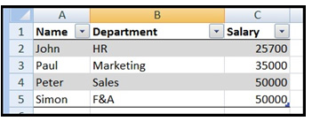
=Vlookup(“Simon”, A1:C5, 3, False) will look for the exact value “Simon” in column A and return the value in the 3rd column; this value is 50000.
=Vlookup(“P”, A1:C5, 2, True) will first look for an exact match; as there is not an exact match then it will look for the next lowest value which is lower than “P”, in this case “John”, and return the value in the 2nd column; this value is HR.
Conclusion
Vlookup, if used correctly, is a powerful function that allows Microsoft Excel to function as a rudimentary relational database. With Vlookup you are able to link different tables of data using common information therefore reducing the need for duplication of information.